Assignment - Machine Learning for Signal Processing

Problem 1: Instantaneous Source Separation

1. As you might have noticed from my long hair, I've got a rock spirit. However, for this homework I dabbled to compose a piece of music that is jazzy. The title of the song is boring: Homework 3.

2. From x_ica_1.wav to x_ica 20.wav are 20 recordings of my song, Homework 3. Each recording has N time domain samples. In this music there are K unknown number of musical sources played at the same time. In other words, as I wanted to disguise the number of sources, I created unnecessarily many recordings of this simple music. This can be seen as a situation where the source was mixed up with a 20 × K mixing matrix A to the K sources to create the 20 channel mixture:

3. But, as you've learned how to do source separation using ICA, you should be able to separate them out into K clean speech sources.

4. First, you don't like the fact that there are too many recordings for this separation problem, because you have a feeling that the number of sources is a lot smaller than 20. So, you decided to do a dimension redcution first, before you actually go ahead and do ICA. For this, you choose to perform PCA with whitening option. Apply your PCA algorithm on your data matrix X, a 20 × N matrix. Don't forget to whiten the data. Make a decision as to how many dimensions to keep, which will correspond to your K. Hint: take a very close look at your eigenvalues.

5. On your whitened/dimension reduced data matrix Z (K ×N), apply ICA. At every iteration of the ICA algorithm, use these as your update rules:

ΔW ← (NI - g(Y)f(Y)')W

W ← W + ρΔW

Y ← WZ

where

W: The ICA unmixing matrix you're estimating

Y: The K × N source matrix you're estimating

Z: Whitened/dim reduced version of your input (using PCA)

g(x): tanh(x)

f(x): x³

ρ: learning rate

N: number of samples

6. Enjoy your separated music. Submit your separated .wav files, source code, and the convergence graph.

7. Implementation notes: Depending on the choice of the learning rate the convergence of the ICA algorithm varies. But I always see the convergence in from 5 sec to 90 sec in my iMac.

Problem 2: Single-channel Source Separation

1. You can use a variety of error functions for the NMF algorithm. An interesting one is to see the matrices as a probabilistic distribution though not normalized. I actually prefer this one than the one I introduced in L6 S35. From this, you can come up with this error function:

ε(X||WH) = ∑_i,j X_i,j log(X_i,j/X^{^}_i,j) - X_i,j + X^{^}_i,j,  (2)

where Xˆ = WH. I wouldn't bother you with a potential question that might ask you to derive the update rules. Instead, I'll just give them away here:

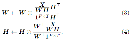
Note that 1^FxT is a matrix full of ones, whose size is F x T, where F and T are the number of rows and columns of your input matrix X, respectively. Please note that, once again, we have multiplicative update rules. Therefore, once you initialized your parameter matrices W and H with nonnegative random values, you can keep their non-negativity as long as your input matrix X is nonnegative as well.

2. trs.wav is a speech signal of a speaker. Load it and convert it into the time-frequency domain by using STFT. For STFT, take a frame of 1024 samples with 50% overlap. Use Hann windows. This will give 1024 × 990 complex-valued matrix (You could get slightly more or less columns than mine depending on your STFT setup). From homework 1 problem 1, you should have noticed that this kind of matrix has complex conjugacy: bottom half of the spectrogram is a mirrored version of the upper half. This is because of the fact that cos(θ) = cos(2π - θ) (the real part) and sin(θ) = - sin(2π - θ) (the imaginary part). Discard the complex conjugate part (the bottom half). So eventually it will be an 513 × 990 matrix. Later on in this problem when you recover the time domain signal out of this, you can easily recover the discarded half from the existing half so that you can do inverse-DFT on the column vector of full 1024 points. Hint: Why 513, not 512? Create a very short random signal with 16 samples, and do a DFT transform to convert it into a spectrum of 16 complex values. Check out their complex coefficients to see why you need 1024/2 + 1, not 1024/2.

3. Take the magnitudes of this matrix. Let's call these magnitudes S, which is nothing but a matrix of nonnegative elements. Learn an NMF model out of this such as S ≈ W_SH_S using the update rules (3) and (4). You know, WS is a set of basis vectors. If you choose to learn this NMF model with 30 basis vectors, then W_S ∈ R^513×30₊, where R₊ is a set of nonnegative real numbers. You're going to use W_S for your separation.

4. Repeat this process for your another training signal trn.wav. Learn another NMF model from trn.wav, which is another training signal for your noise. From this get W_N.

5. x_nmf.wav is a noisy speech signal made of the same speaker's different speech and the same type of noise you saw. By using our third NMF model, we're going to denoise this one. Load this signal and convert it into a spectrogram X ∈ C^513×131. Let's call its magnitude spectrogram Y = |X| ∈ R^513×131₊. Your third NMF will learn this approximation:

Y ≈ [W_SW_N]H. (5)

What this means is that for this third NMF model, instead of learning new basis vectors, you reuse the ones you trained from the previous two models as your basis vectors for testing: W = [W_SW_N]. As you are very sure that the basis vectors for your test signal should be the same with the ones you trained from each of the sources, you initialize your W matrix with the trained ones and don't even update it during this third NMF. Instead, you learn a whole new H ∈ R^60×131₊ that tells you the activation of the basis vectors for every given time frame. Implementation is simple. Skip the update for W. Update H by using W = [W_SW_N] and Y. Repeat. Note: You're doing a lot of element-wise division, so be careful not to divide by zero. To prevent this, I tend to add a very small value (e.g. eps in MATLAB) to every denominator element in the update rule.

6. Because W_SH_(1:30,:) can be seen as the speech source estimate, you can also create a magnitude masking matrix out of it:

M¯ = W_SH_(1:30,:)/(W_SH_(1:30,:) + W_NH_(31:60,:)) = W_SH_(1:30,:)/[W_SW_N]H. (6)

Use this masking matrix to recover your speech source, i.e. Sˆ = M¯ X. Recover the bottom 511 rows by using the conjugacy discussed in 2. Invert back to the time domain. Listen to it to see if the noise is suppressed.

Submit the wav file and source code.

Problem 3: Motor Imagery

1. eeg.mat has the training and testing samples and their labels. Use them to replicate my BCI classification experiments in Module 5 (not the entire lecture, but from S3 to S8 and S37). But, instead of PCA dimension reduction, we're going to use locality sensitive hashing to extract binary features. Also, instead of naive Bayes, we'll do kNN classification.

2. For the kNN classification, for every test example you have to find the K nearest neighbors from 112 training samples. You're lucky. This kNN search is not a big deal, because your training set is tiny. However, as your professor I have to help you guys be prepared for your future big data projects at your fancy new job after your graduation (don't forget me). So, I'm giving you this homework assignment that will help you come up with a speed-up technique for the kNN search. It's not that complicated.

3. Come up with a random projection matrix A ∈ R^L×M, where M denotes the number of dimensions of your data samples (5 rows of your magnitude STFT, vectorized), 255, and L is the new dimension after this random projection. So, you're replacing PCA with this random projection. Note that L doesn't always have to be smaller than M. Although A is a matrix with random values, you should make sure that the row vectors (the projection vectors) should be unit vectors, i.e. ||A_i,:||2 = 1. Make sure of it.

4. Do the random projection and take the sign of the result (element-wise), so that your random projection produces a bunch of +1's and -1's:

Y = sign(AZ_1:M,:) (7)

5. Use this A matrix and the sign function wrapper to convert your 255 dimensional TRAINING samples into L-dimensional bipolar binary hash codes. Ditto for the TEST samples (use the same A matrix). If you're not comfortable with bipolar binaries, you can turn them into 0-1 binaries by replacing -1's with 0's. It's up to you.

6. Do your kNN classification using these binary version of your data samples. Note that you can compare the test bit string with the bit strings of the training data by using the Hamming distance, instead of the Eucleadian distance between the original real-valued vectors. You know your computer prefers binary values, right? This way you can speed up the comparison, and eventually the kNN search (although you might not be able to see the actual speed-up due to the too small dataset size and your script language that doesn't exploit binary variables). Report your classification results with different choice of K, L and M. I think a table of accuracies will be great. You don't have to submit all the intermediate plots. What I need to see is the accuracies and your source code.

7. Compare your results with mine in M5 S37. You're classifier is based on binary variables and bitwise operations, so you must have expected a big performance drop. How do you like it eventually? Report your classification accuracy. Submit your code and your discussion.

Problem 4: kNN Source Separation

1. Prepare your S and N matrices by using the procedure in 2.2-2.4, but without NMF, i.e. they are the input magnitude spectrogram to your NMF. This time, let's create another matrix G, the magnitude spectrogram of trs.wav+trn.wav. Also, let's create another matrix called Ideal Binary Masks (IBM), B defined as follows:

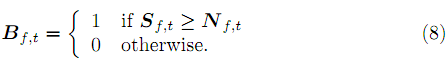
My hope is that S ≈ B G. This sounds a bit too rough, but it actually works well, because if you take a look at the local bins, they are dominated by one of the sources, not really all of them due to the sparsity of the sources in the TF domain. If you can't believe in me, go ahead and convert S back to the time domain (with proper phase information) to check out the sound, although I don't require it.

2. Load x_nmf.wav and convert it into X and Y like in 2.5. We're not doing NMF on this though. This time, we compare each column of Y with all columns in G to find out k nearest neighbors. Then, for t-th given test frame, we have a list of indices to the k nearest frames in G, e.g. {i₁, i₂, · · · , i_k}, where i₁, i₂, · · · , i_k ∈ {1, · · · , 990}. For the comparison, I used Euclidean distance for no good reason, but you can choose a different (more proper) one if you want.

3. What we want to do with this is to predict the IBM of the test signal, D ∈ B^513×131. By using the nearest neighbor indices, I can collect the IBM vectors from B, i.e. {B_:,i1, B_:,i2, · · · , B_:,ik}. Since Y_:,t is very similar to {G_:,i1, G_:,i2, · · · , G_:,ik}, I hope that my D_:,t should be similar to {B_:,i1, B_:,i2, · · · , B_:,ik}. How do we consolidate them though? Let's try median of them, because that'll give you one if one is the majority, and vice versa:

D_:,t = median({B_:,i1, B_:,i2, · · · , B_:,ik}). (9)

4. Repeat this for all your test frames (131 frames in my STFT) and predict the full D matrix. Recover the complex-valued spectrogram of your speech by masking the input: Sˆ_test = D X. Convert it back to the time domain. Listen to it. Is the noise suppressed? Submit this wavefile as well as your code.

Attachment:- Assignment Files - Advanced Machine Learning.rar