Transfer Functions

1. Assume that the unit step response of a linear time-invariant system is given by

c(t) = 1 + e^-tcos(t) + e^-2t sin(3t), t ≥ 0.                       (1)

(a) Obtain the transfer function of the system.

(b) Determine the zeros and poles of the system.

Linearization of Nonlinear Dynamical Systems

2. Consider a 1 (kg) mass connected to a nonlinear damper and spring whose forces are given by 2 tanh(x^·)  and 2 tan^-1(x), respectively, in which x and x^· represent the horizontal position (m) and velocity (m/s) of the mass. Then, the dynamical equation of motion can be given by

x¨ + 2 tanh(x^·) + 2 tan^-1(x) = u,                                   (2)

where u denotes the external force applied to the mass.

(a) Present a state-space equation for the dynamical system in (2).

(b) Using MATLAB/Simulink, obtain the system response for a step input with the magnitude 0.1 (N) and initial conditions being x(0) = 0 (m) and x^·(0) = 0 (m/s) over the time interval [0, 10](s).

(c) Obtain the linearized model of (2) around x = 0 (m) and x^· = 0 (m/s).

(d) Using MATLAB/Simulink, obtain the response of the linearized system for a step input with the magnitude 0.1 (N) and initial conditions being zero over the time interval [0, 10](s).

(e) Plot the responses of the linearized and nonlinear systems together and compare the solutions. What do you conclude?

Mathematical Modeling

3. Consider the dynamical system of Fig. 1, in which x1 and x2 represent the vertical displacements of masses m₁ and m₂ with respect to the ground, respectively. Let u denote the external force applied to mass m₁. Assume that m₁ = 10 (kg) m₂ = 0.1 (kg), and k₁ = k₂ = 10 (N/m).

Remark: Do not consider the gravity terms.

(a) Present a state-space equation for the dynamical system in Fig.1.

(b) Using MATLAB/Simulink, plot the system response for a step input with the magnitude 0.1(N), and initial conditions x₁(0) = 0.1 (m), x₂(0) = -0.1 (m), x^·₁(0) = x^·₂(0) = 0 (m/s) over the time interval [0, 10](s).

(c) Obtain the transfer functions x₁(s)/u(s) and x₂(s)/u(s). Compute the zeros and poles of these transfer functions.

Second-Order Systems

4. Consider a rigid body with the moment of inertia J rotating around a fixed axis. Let θ, ω = θ? and u represent the angular position and velocity of the body, and the external torque applied to the body, respectively. Here, we assume that there are no rotational friction and compliance in this motion. To stabilize the position of the body, we employ a control system as shown in Fig. 4. The closed-loop system includes position and velocity loops with gains K_p and K_v, respectively.

(a) Obtain the closed-loop transfer function θ(s)/r(s), where r(s) is the set-point for the position.

(b) Assume that J = 1 (kgm²). Design K_p and K_v such that the maximum overshoot and the peak time for the unit step response become 0.2 and 1 (s), respectively.

Design of a PID Controller for the Ball and Beam System

5. Physical Setup: A ball is placed on a beam, see figure below, where it is allowed to roll with 1 degree of freedom along the length of the beam. A lever arm is attached to the beam at one end and a servo gear at the other. As the servo gear turns by an angle θ, the lever changes the angle of the beam by α. When the angle is changed from the horizontal position, gravity causes the ball to roll along the beam. A controller will be designed for this system so that the ball's position can be manipulated.

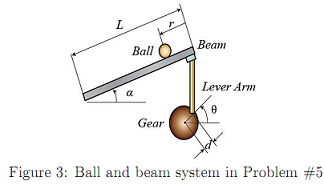
System Parameters: For this problem, we will assume that the ball rolls without slipping and friction between the beam and ball is negligible. The constants and variables for this problem are defined as follows:

(m) mass of the ball = 0.11 (kg)

(R) radius of the ball = 0.015 (m)

(d) lever arm offset = 0.03 (m)

(g) gravitational acceleration =9.8 (m/s²)

(L) length of the beam =1.0 (m)

(J) ball's moment of inertia = 9.99 × 10^-6(kg.m²)

(r) ball position coordinate

(α) beam angle coordinate

(θ) servo gear angle

System Equations: The second derivative of the input angle α actually affects the second derivative of r. However, we will ignore this contribution. The Lagrangian equation of motion for the ball is then given by the following:

0 = (J/R² + m)r^·· + mg sinα - mrα^·2                (3)

Linearization of this equation about the beam angle, α = 0, gives us the following linear approximation of the system:

(J/R² + m)r¨ = -mgα                                        (4)

The equation which relates the beam angle to the angle of the gear can be approximated as linear by the equation below:

α = (d/L)θ                                                        (5)

Substituting this into the previous equation, we get:

(J/R² + m)r¨ = -mg(d/L)θ                                 (6)

• By taking the Laplace transform of the equation (6), obtain the transfer function of the open-loop system, defined as, G(s) := r(s)/θ(s). Here, the servo gear angle θ is assumed to be the control input for the open-loop system.
• Design a unity closed-loop control system with the desired input rd (i.e., desired ball position) and the actual output r (i.e., actual ball position) using a PID controller to achieve the following requirements: (1) Settling time < 3 seconds, and (2) Overshoot < 5%.
• Using MATLAB/Simulink, simulate the linear closed-loop system's response for a step input 0.1 (m) in the presence of a step-like external disturbance with the magnitude 5π/180 (rad) over the time interval [0, 10] (s).
• Using final value theorem, compute the final value of the closed-loop output, i.e., lim_t→∞ r(t), for a ramp input in the absence of the external disturbance. Repeat this computation for an acceleration input. Check your results with MATLAB/Simulink.

Design of a PID Controller for an Aircraft Pitch System

5. Physical Setup: The equations governing the motion of an aircraft are a very complicated set of six nonlinear coupled differential equations. However, under certain assumptions, they can be decoupled and linearized into longitudinal and lateral equations. Aircraft pitch is governed by the longitudinal dynamics. In this problem, we will design an autopilot that controls the pitch of an aircraft.

The basic coordinate axes and forces acting on an aircraft are shown in the figure given below.

We will assume that the aircraft is in steady-cruise at constant altitude and velocity; thus, the thrust, drag, weight and lift forces balance each other in the x- and y-directions. We will also assume that a change in pitch angle will not change the speed of the aircraft under any circumstance (unrealistic but simplifies the problem a bit). Under these assumptions, the longitudinal equations of motion for the aircraft can be written as follows:

α^· = -0.313α + 56.7q + 0.232δ                                   (7)

q^· = -0.0139α - 0.426q + 0.0203δ                               (8)

θ^· = 56.7q.                                                               (9)

For this system, the input will be the elevator deflection angle δ and the output will be the pitch angle θ of the aircraft. The numerical values are taken from the data from one of Boeing's commercial aircraft.

• By taking the Laplace transform of the above equations, obtain the transfer function of the open-loop system, defined as, G(s) := θ(s)/δ(s).
• Design a unity closed-loop control system with the desired input θ_d (i.e., desired pitch position) and the actual output θ (i.e., actual pitch position) using a PID controller to achieve the following requirements: (1) Settling time < 10 seconds, and (2) Overshoot < 10%.
• Using MATLAB/Simulink, simulate the closed-loop system's response for a step input 0.1 (rad) in the presence of a step-like external disturbance with the magnitude -6π/180 (rad) over the time interval [0, 20] (s).
• Using final value theorem, compute the ?nal value of the closed-loop output, i.e., lim_t→∞ θ(t), for a ramp input in the absence of the external disturbance. Check your results with MAT-LAB/Simulink.

Attachment:- Assignment Files.rar