Let's start by loading the data file included with this empirical exercise into Gretl. The filename is "gretl_ex2_gasoline.xls". First, save this file to your computer being sure to keep it in .xls format. Then import this data file into Gretl using the instructions in Empirical Exercise 1 (if you have forgotten). Gretl will recognize the first column as the year variable, and tell you so; that's okay, click "close".

We have loaded time series data related to the U.S. gasoline market from 1953 - 2004. The variable definitions are as follows:

• Year = Year, 1953-2004
• GasExp = total U.S. gasoline expenditure in billions of U.S. dollars
• Pop = U.S. total population in thousands
• GasP = Price index for gasoline
• Income = Per capita disposable income
• PNC = Price index for new cars
• PUC = Price index for used cars
• PPT= Price index for public transportation
• PD = Aggregate price index for consumer durables
• PN = Aggregate price index for consumer nondurables
• PS = Aggregate price index for consumer services

Our first task is to generate a new variable. We want to calculate real per capita gasoline expenditures, so

RealGasCap = GasExp/ Pop * GasP

In Gretl this can be done by clicking, Add > Define New Variable. You will see the following window

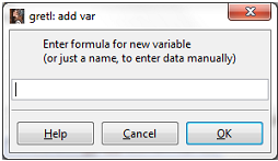
Enter the following formula: RealGasCap = GasExp/(Pop*Gasp), and click OK. You will see that new variable has been generated and is listed in your variable list.

OLS Estimation of Regression Coefficients Using Gretl

I will quickly show you how to run an OLS regression in Gretl, and then I'll ask you to run a few more regressions and interpret the results.

First, click Model > Ordinary Least Squares. The following window will appear:

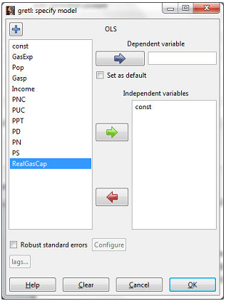
Click on "RealGasCap" so that it is highlighted then click the blue arrow to select per capita gasoline expenditures as the dependent variable (Y). Next, click on "Gasp" and click on the green arrow to select the gasoline price index as the independent variable (X). Gretl
automatically includes a constant term in the regression ("const"). Once you have done this, click OK.

So, we have estimated the following two-variable model:

RealGasCap_t = β₁ + β₂Gasp_t + u_t

What is your expectation about the sign of β₂? According to microeconomic theory, the law of demand tells us that β₂ should be negative. An increase in the price of gasoline will lead to a decrease in the quantity demanded of gasoline (real per capita expenditures).

Let's look at the results to find out: (I copied (by right-clicking and selecting "copy") the Gretl results in RTF (MS Word) format and pasted them below - this seems to be the best option.)

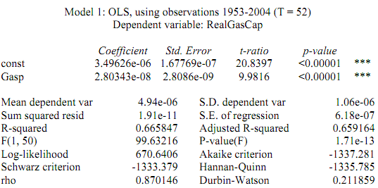
What happened? We obtain a statistically significant slope coefficient equal to 0.000000028, implying that a one unit increase in the gasoline price index will lead to a 0.000000028 billion dollar increase in real per capita gasoline expenditures (recall that expenditures are measured in billions of dollars). So in other words, a one unit increase in in the gasoline price index will lead to a 28 dollar increase in real per capita gasoline expenditures. We can also see the calculated
 (coefficient of determination) is equal to 0.6658 meaning that around 67% of the variation in real per capita gasoline expenditures is explained by the gasoline price index.

Have we just proven that the law of demand does not hold for gasoline? Not so fast. First of all, while this result is statistically significant; is it economically significant? Obviously, there are many other things that may be impacting the demand for gasoline besides its own price. So we will estimate this model in a multiple regression context and estimate different demand elasticities on Homework 3; but for now, let's just run a few more two-variable regressions to develop our intuition about some of these expected relationships.

NOTE that the price variables included in this data set are price indices, NOT the actual prices of the various commodities over time! In other words, the price variables are NOT measured in dollars. Since they are indices, they have no units; but they do tell us how prices are changing over time.

EXERCISES:

1. Setup a two-variable regression model (i.e. write down the PRF) to examine the impact of per capita disposable income on real per capita gasoline expenditures.

a. Based off your know knowledge of microeconomic theory, what are your expectations about the sign of β₂? Why?
b. Estimate the model. Display your regression results.

c. Is β₂ statistically significant? How do you know?

d. Comment on the sign of β₂. Does this align with your expectations? Provide an interpretation of the slope coefficient .

2. Setup a two-variable regression model (i.e. write down the PRF) to examine the impact of the price of public transportation on real per capita gasoline expenditures.

a. Based off your knowledge of microeconomic theory, what are your expectations about the sign of β₂? Why?

b. Estimate the model. Display your regression results.

c. Is β₂ statistically significant? How do you know?

d. Comment on the sign of β₂. Does this align with your expectations? Provide an interpretation of the slope coefficient β₂.

Attachment:- Empirical-exercise-2-Econometrics.xlsx